Continuous Control with
Action Quantization from Demonstrations

Introduction

Reinforcement Learning (RL) relies on Markov Decision Processes (MDP) as its cornerstone, a general framework under which vastly different problems can be casted. There is a clear separation in the class of MDPs between the finite discrete action setup, where an agent faces a finite number of possible actions, and the continuous action setup, where an agent faces an infinite number of actions. The former is arguably simpler, since exploration is more manageable with a finite number of actions, and computing the maximum of the action-value function is straightforward (and implicitly defines a greedily-improved policy). In the continuous action setup, the parametrized policy either directly optimizes the expected value function that is estimated through Monte Carlo rollouts, which makes it demanding in interactions with the environment, or tracks the maximum of the bootstrapped value function hence introducing additional sources of approximations.

Therefore, a natural workaround consists in turning a continuous control problem into a discrete one. The simplest approach is to naively (uniformly) discretize the action space, an idea which dates back to the "bang-bang" controller. However, such a discretization scheme suffers from the curse of dimensionality. A number of methods have addressed this limitation by making causal dependence assumptions between the different action dimensions, but they are typically complex and task-specific.

We thus propose Action Quantization from Demonstrations, or AQuaDem, a novel paradigm where we learn a state dependent discretization of a continuous action space using demonstrations, enabling the use of discrete-action deep RL methods by virtue of this learned discretization. We formalize this paradigm, provide a neural implementation and analyze it through visualizations in simple grid worlds. We empirically evaluate this discretization strategy on three downstream task setups: Reinforcement Learning with demonstrations, Reinforcement Learning with play data, and Imitation Learning. We test the resulting methods on manipulation tasks and show that they outperform state-of-the-art continuous control methods both in terms of sample-efficiency and performance on every setup.

Method

The AQuaDem framework quantizes a continuous action space conditionally on the state, from a dataset of demonstrations \mathcal{D} . Formally, the goal is to learn a function \Psi: s \in \mathcal{S} \mapsto (\Psi_1(s), ..., \Psi_K(s)) \in \mathcal{A}^K , that takes a state as an input and outputs K action candidates. When this mapping is learned (fully offline), we can learn a controller uniquely on a discrete action space (using a discrete deep RL method e.g. DQN), which consists in executing one of the K actions candidates. We propose the following objective to learn the quantization mapping (where T is a hyperparameter):

\min_{\Psi} \mathbb{E}_{s, a \sim \mathcal{D}} \Big[ - \log \Big( \sum^K_{k=1} \exp\big( \frac{-\|\Psi_k(s) - a \|^2}{T}\big) \Big) \Big].

This equation corresponds to minimizing a soft-minimum of the distances between the candidate actions \Psi_1(s), ..., \Psi_K(s) and the demonstrated action a . Note that with K=1, this is exactly the BC loss. The larger the temperature T is, the more the loss imposes all candidate actions to be close to the demonstrated action a thus reducing to the BC loss. The lower the temperature T is, the more the loss only imposes a single candidate action to be close to the demonstrated action a.

Why Discretize?

The choice of reducing the action space to a few actions is somewhat counterintuitive, as it constrains the family of policies for the problem (and might exclude near-optimal policies). Nevertheless, this discretization strategy has the benefit of 1) turning a continuous action problem into a discrete one 2) constraining the possible actions to be close to the one taken by the demonstrator (which supposedly are good). The reason why discrete action spaces are arguably preferable is that they enable the exact computation of the maximum of the approximate action-value function. In the continuous action setting, state of the art methods such as SAC or TD3 introduce a policy that approximately tracks the maximum of the approximate action-value function.

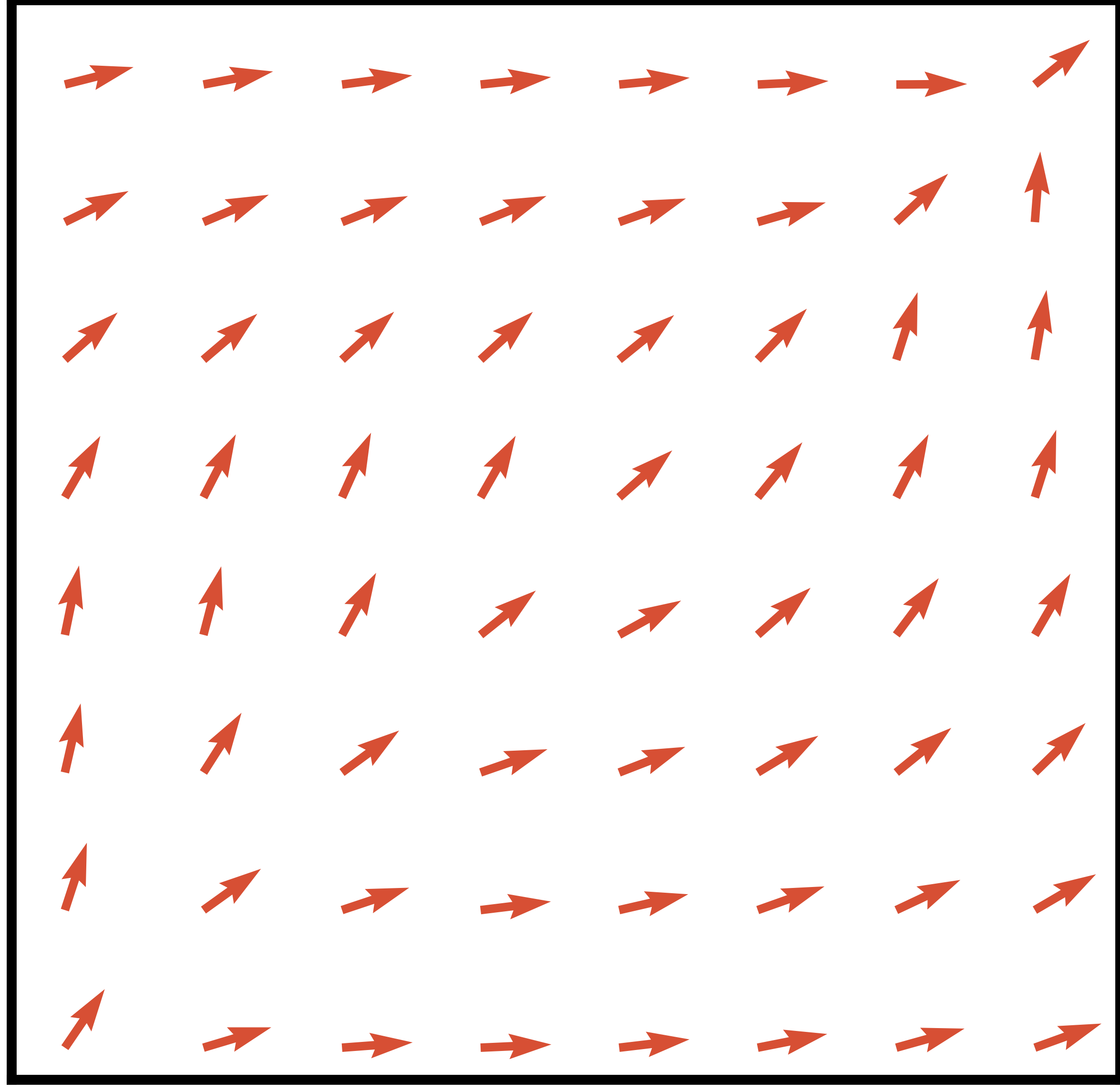
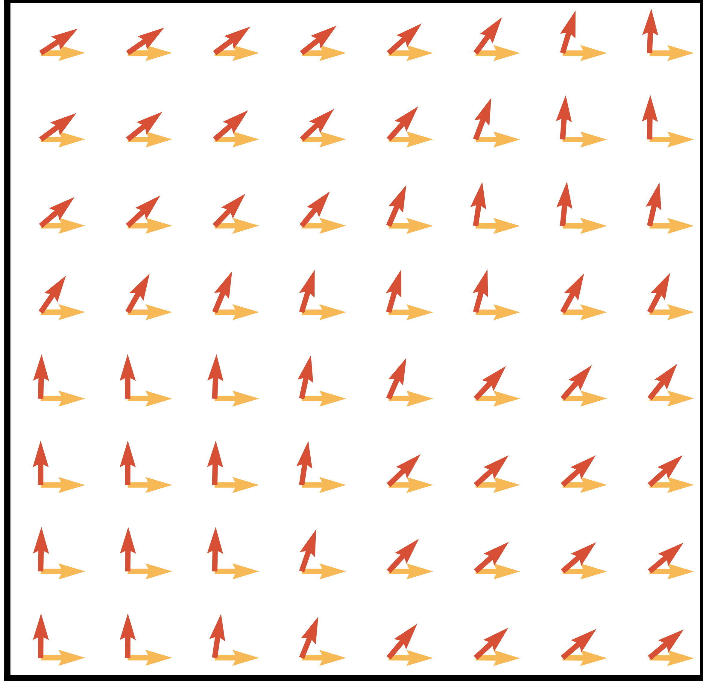
Action Candidates Visualization: a continuous navigation gridworld.

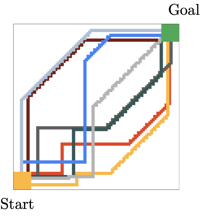We introduce a grid world environment where the start state is in the bottom left, and the goal state is in the top right. Actions are continuous (2-dimensional), and give the direction in which the agent take a step. These steps are normalized by the environment to have fixed L2 norm. The stochastic demonstrator moves either right or up in the bottom left of the environment then moves diagonally until reaching the edge of the grid, and goes either up or right to reach the target. The demonstrations are represented in the different colors.

We define a neural network \Psi and optimize its parameters by minimizing the AQuaDem objective function. We display the resulting candidate actions across the state space below as a function of the number of action candidates and the temperature T. As each color of the arrows depicts a single head of the \Psi network, we observe that the action candidates are smooth: action candidates slowly vary as the state varies, which prevents to have inconsistent action candidates in nearby states. Note that BC actions tend to be diagonal even in the bottom left part of the action space, where the demonstrator only takes horizontal or vertical actions. On the contrary, the action candidates learned by AQuaDem include the actions taken by the demonstrator conditioned on the states.

Behavioral Cloning Actions

AQuaDem Candidates Actions

K 2 3 Temperature 0.001 0.01 0.1 1.0

Action Candidates Visualization: a door opening task.

We represent the actions candidates learned using the AQuaDem framework on the Door environment which comes with 25 demonstrations of the task. As the action space is of high dimensionality, we choose to represent each action dimension on the x-axis, and the value for each dimension on the y-axis. We connect the dots on the x-axis to facilitate the visualization through time. We replay trajectories from the human demonstrations and show at each step the 10 actions proposed by the AQuaDem network, and the action actually taken by the human demonstrator. Each action candidate has a color consistent across time (meaning that the blue action always correspond to the same head of the \Psi network). Interestingly, the video shows that actions are very state dependent (except some default 0-action) and that they evolve smoothly through time.

Reinforcement Learning with Demonstrations

Setup. In the Reinforcement Learning with demonstrations setup (RLfD), the environment of interest comes with a reward function and demonstrations (which include the reward), and the goal is to learn a policy that maximizes the expected return. This setup is particularly interesting for sparse reward tasks, where the reward function is easy to define (say reaching a goal state) and where RL methods typically fail because the exploration problem is too hard. We consider the Adroit tasks, for which human demonstrations are available (25 episodes acquired using a virtual reality system). These environments come with a dense reward function that we replace with the following sparse reward: 1 if the goal is achieved, 0 otherwise.

Algorithm & baselines. The algorithm we propose is a two-fold training procedure: 1. we learn a quantization of the action space using the AQuaDem framework from human demonstrations; 2. we train a discrete action deep RL algorithm on top of this this quantization. We refer to this algorithm as AQuaDQN. The RL algorithm considered is Munchausen DQN. To make as much use of the demonstrations as possible, we maintain two replay buffers: one containing interactions with the environment, the other containing the demonstrations that we sample using a fixed ratio similarly to DQfD. We consider SAC and SAC from demonstrations (SACfD) --a modified version of SAC where demonstrations are added to the replay buffer-- as baselines against the proposed method. The hyperparameter search of the proposed method and the baselines used the same amount of compute and are detailed here: AQuaDQN, SACfD, SAC. We do not include naive discretization baselines, as the dimension of the action space is at least 24, which would lead to ~16M actions with a binary discretization scheme.

Evaluation & results. We train the different methods on 1M environment interactions on 10 seeds for the chosen hyperparameters (a single set of hyperameters for all tasks) and evaluate the agents every 50k environment interactions (without exploration noise) on 30 episodes. An episode is considered a success if the goal is achieved during the episode. The AQuaDem discretization is trained offline using 50k gradient steps on batches of size 256. The number of actions considered were 10,15,20 and we found 10 to be performing the best. The Figure below shows the returns of the trained agents as well as their success rate. On Door, Pen, and Hammer, the AQuaDQN agent reaches high success rate, largely outperforming SACfD in terms of success and sample efficiency.

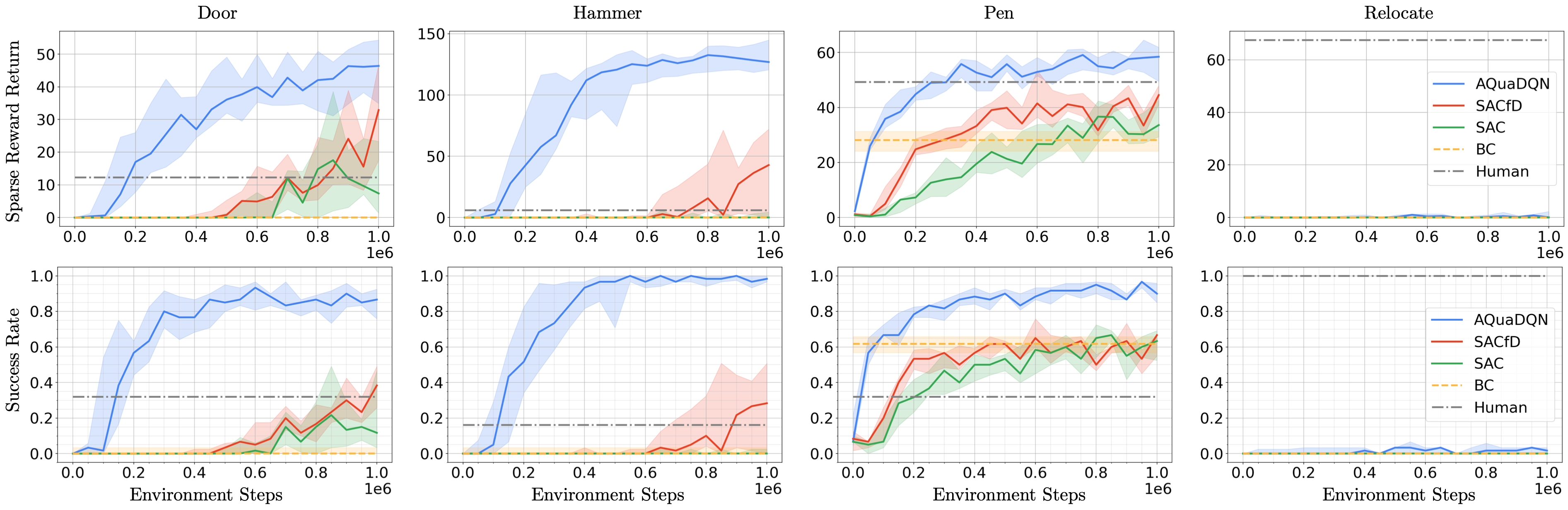
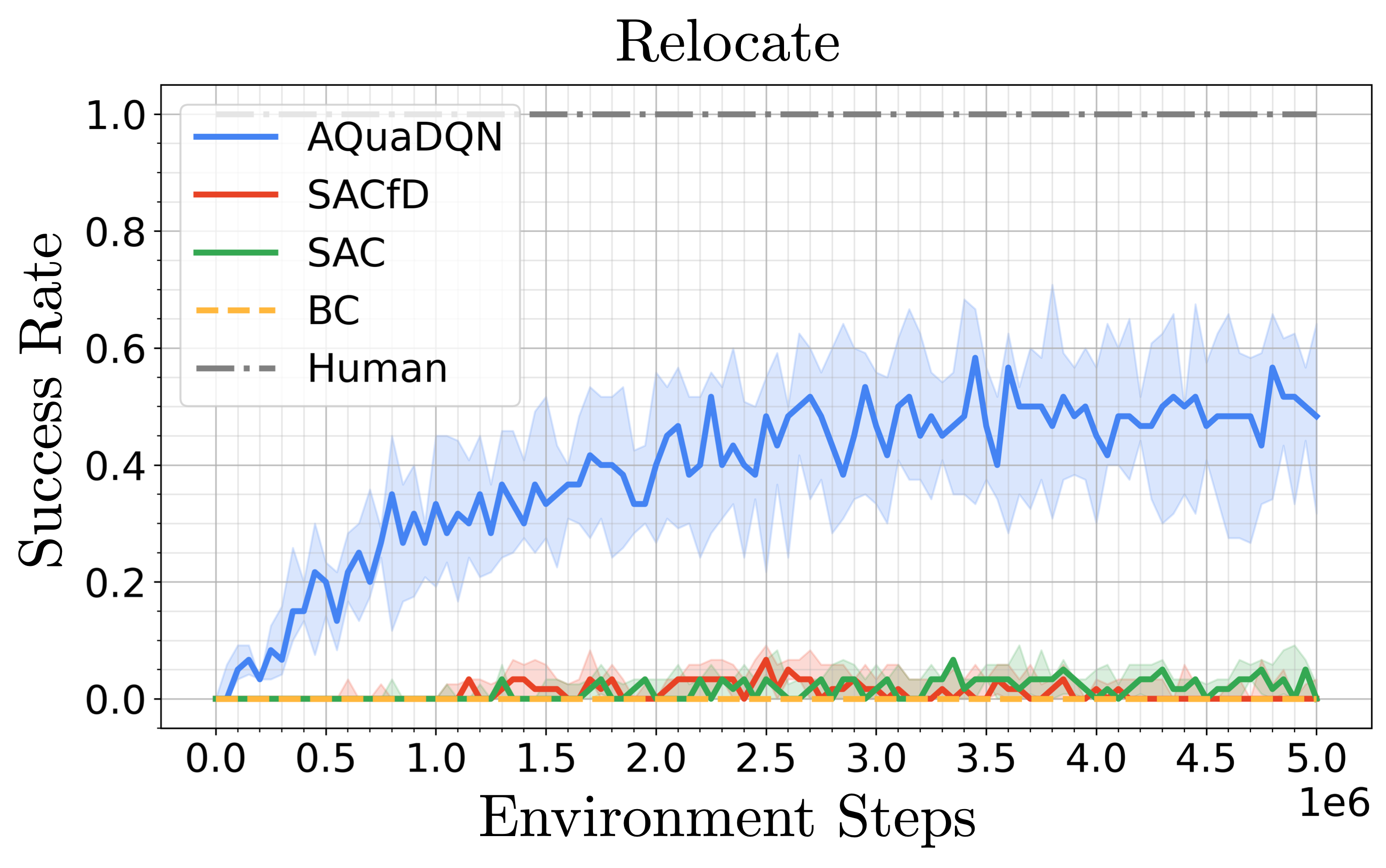On Relocate, all methods reach poor results (although AQuaDQN slightly outperforms the baselines). The task requires a larger degree of generalisation than the other three since the goal state and the initial ball position are changing at each episode. However, we show below that when tuned uniquely on the Relocate environment and with more environment interactions, AQuaDQN manages to reach a 50% success rate where other methods still fail. Notice that on the Door environment, the SAC and SACfD agents outperform the AQuaDQN agent in terms of final return (but not in term of success rate). The behavior of these agents are however different from the demonstrator since they consist in slapping the handle and abruptly pulling it back. We provide videos of all resulting agents below (one episode for each seed which is not cherry picked) to demonstrate that AQuaDQN consistently learns a behavior that is qualitatively closer to the demonstrator.

Imitation Learning

Setup. In Imitation Learning, the task is not specified by the reward function but by the demonstrations themselves. The goal is to mimic the demonstrated behavior. There is no reward function and the notion of success is ill-defined. Imitation Learning is of particular interest when designing a satisfying reward function --one that would lead the desired behavior to be the only optimal policy-- is harder than directly demonstrating this behavior. In this setup, there is no reward provided, not in the environment interactions nor in the demonstrations. We again consider the Adroit environments and the human demonstrations which consist of 25 episodes acquired via a virtual reality system.

Algorithm & baselines. Again, the algorithm we propose has two stages: 1) we learn --fully offline-- a discretization of the action space using AQuaDem, 2) we train a discrete action version of the GAIL algorithm in the discretized environment. More precisely, we interleave the training of a discriminator between demonstrations and agent experiences, and the training of a Munchausen DQN agent that maximizes the confusion of this discriminator. The Munchausen DQN takes one of the candidates actions given by AQuaDem. We call this algorithm AQuaGAIL. As a baseline, we consider the GAIL algorithm with a SAC agent directly maximizing the confusion of the discriminator. This results in a very similar algorithm as the one proposed by. We also include the results of BC. The hyperparameter search of the proposed method and the baselines used the same amount of compute and are detailed here: AQuaGAIL, GAIL, BC.

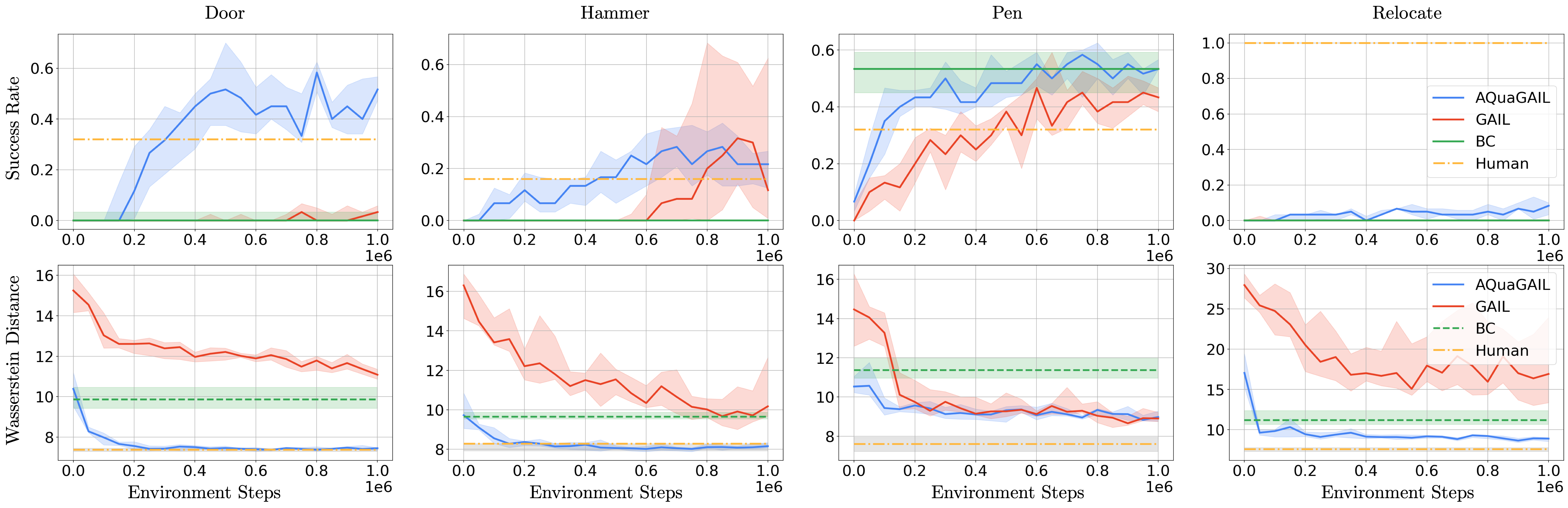
Evaluation & results. We train AQuaGAIL and GAIL for 1M environment interactions on 10 seeds for the selected hyperparameters (a single set for all tasks). BC is trained for 60k gradient steps with batch size 256. We evaluate the agents every 50k environment steps during training (without exploration noise) on 30 episodes. The AQuaDem discretization is trained offline using 50k gradient steps on batches of size 256. Evaluating imitation learning algorithms has to be done carefully as the goal to "mimic a behavior" is ill-defined. Here, we provide the results according to two metrics. On top, the success rate (notice that the human demonstrations do not have a success score of 1 on every task). We see that, except for Relocate, which is a hard task to solve with only 25 human demonstrations due to the necessity to generalize to new positions of the ball and the target, AQuaGAIL solves the tasks as successfully as the humans, outperforming GAIL and BC. Notice that our results corroborate previous work that showed poor performance of GAIL on human demonstrations after 1M steps. The second metric we provide, on the bottom, is the Wasserstein distance between the state distribution of the demonstrations and the one of the agent. The "human" Wasserstein distance score is computed by randomly taking 5 episodes out of the 25 human demonstrations and compute the Wasserstein distance to the remaining 20. Remark that AQuaGAIL is able to get much closer behavior to the human than BC and GAIL on all four environments in terms of Wasserstein distance. This supports that AQuaDem leads to policies much closer to the demonstrator (which is also demonstrated in the videos).

Reinforcement Learning with Play Data

Setup. The Reinforcement Learning with play data is an under-explored yet natural setup. In this setup, the environment of interest has multiple tasks, a shared observation and action space for each task, and a reward function specific to each of the tasks. We also assume that we have access to play data, introduced by, which consists in episodes from a human demonstrator interacting with an environment with the sole intention to play with it. The goal is to learn an optimal policy for each of the tasks. We consider the Robodesk tasks for which we acquired play data.

Algorithm & baselines. Similarly to the RLfD setting, we propose a two-fold training procedure: 1) we learn a discretization of the action space in a fully offline fashion using the AQuaDem framework on the play data, 2) we train a discrete action deep RL algorithm using this discretization on each tasks. We refer to this algorithm as AQuaPlay. Unlike the RLfD setting, the demonstrations do not include any task specific reward nor goal labels meaning that we cannot incorporate the demonstration episodes in the replay buffer nor use some form of goal-conditioned BC. We use SAC as a baseline, which is trained to optimize task specific rewards. Since the action space dimensionality is fairly low (5-dimensional), we can include naive discretization baselines "bang-bang" (BB) based on different granularities: we refer to them as BB-2, BB-3 and BB-5.

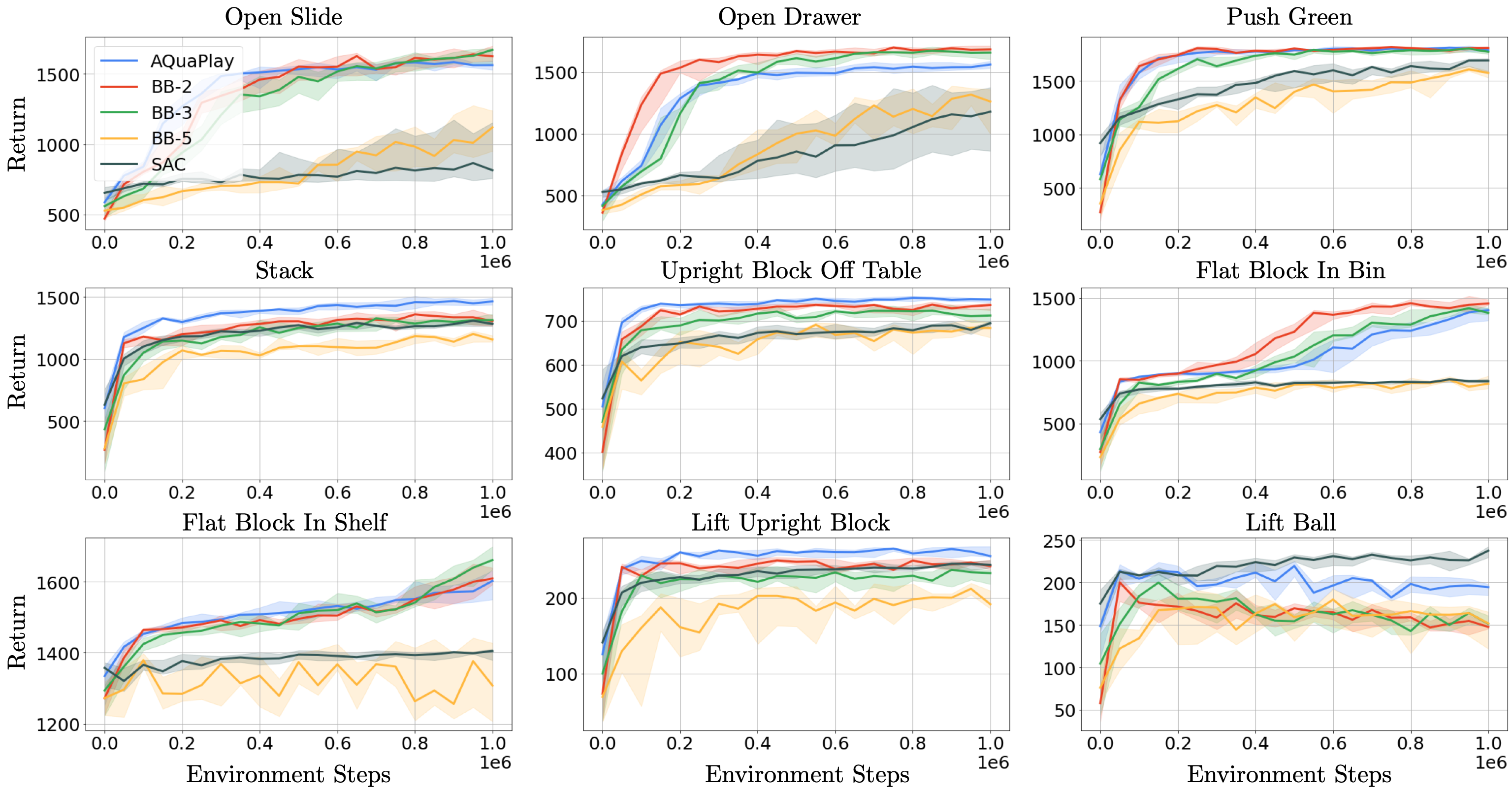
We train the different methods on 1M environment interactions on 10 seeds for the chosen hyperparameters (a single set of hyperameters for all tasks) and evaluate the agents every 50k environment interactions (without exploration noise) on 30 episodes. The AQuaDem discretization is trained offline on play data using 50k gradient steps on batches of size 256. The number of actions considered were 10,20,30,40 and we found 30 to be performing the best. It is interesting to notice that it is higher than for the previous setups. It aligns with the intuition that with play data, several behaviors needs to be modelled. The AQuaPlay agent consistently outperforms SAC in this setup. Interestingly, the performance of the BB agent decreases with the discretization granularity, well exemplifying the curse of dimensionality of the method. In fact, BB with a binary discretization (BB-2) is competitive with AQuaPlay, which validates that discrete action RL algorithms are well performing if the discrete actions are sufficient to solve the task. Note however that the Robodesk environment is a relatively low-dimensional action environment, making it possible to have BB as a baseline, which is not the case of e.g. Adroit where the action space is high-dimensional.

Conclusion

With the AQuaDem paradigm, we provide a simple yet powerful method that enables to use discrete-action deep RL methods on continuous control tasks using demonstrations, thus escaping the complexity or curse of dimensionality of existing discretization methods. We showed in three different setups that it provides substantial gains in sample efficiency and performance and that it leads to qualitatively better agents, as enlightened by the videos. There are a number of different research avenues opened by AQuaDem. Other discrete action specific methods could be leveraged in a similar way in the context of continuous control: count-based exploration, planning or offline RL. Similarly a number of methods in Imitation Learning or in offline RL are evaluated on continuous control tasks and are based on Behavioral Cloning regularization which could be refined using the same type of multioutput architecture used in this work. Another possible direction for the AQuaDem framework is to be analyzed in the light of risk-MDPs as the constraint of the action space arguably reduces a notion of risk when acting in this environment. Finally, as the gain of sample efficiency is clear in different experimental settings, we believe that the AQuaDem framework could be an interesting avenue for learning controllers on physical systems.