Biomaker CA

Disclaimer: this is a web article version of the following paper. The paper contains more technical details and related work. This article is a faster read and presents the content with several videos.

Introduction

This is Biomaker CA.

This project stands for Biome Maker with Cellular Automata. Cellular Automata (CA), because every single cell in the simulation is a (possibly different) CA. Biome, because what you are observing is the simulation of a very simple biome, with energy being generated and dissipated, and 'living' agents trying to survive and reproduce in it. Maker, because, as you will see shortly, this project is not restricted to showing one biome, but its goal is to design and explore as many different biomes as possible, with a small set of laws of physics that can be modified at will.

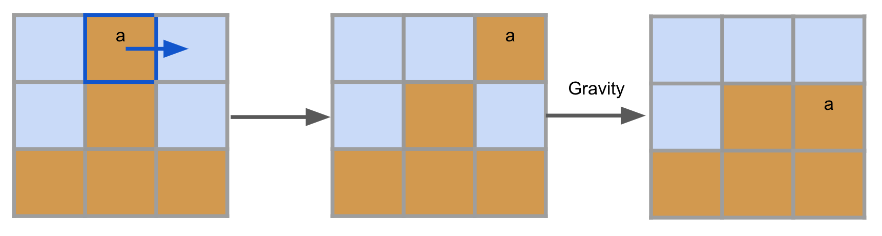
Let us step back a second. Some of you may already be familiar with these kinds of environments, while some of you might still be wondering what is going on. The worlds generated by this project can be categorised into a Falling-sand game. In these games, most if not all of the game logic is based on CA rules being continuously executed and observing complex behaviours emerging from simple rules. Typically, each cell only observes their direct 3x3 neighbourhood and modifies itself and/or its surroundings with some rules based on their cell type. Why are they called falling-sand games? Because "sand" falls and creates heaps, which can be simulated with CA rules:

If you have never played any such games before, we encourage you to spend some time exploring one of the many available falling-sand games (for instance, you could play Sandspiel on your browser) to get a feeling about the power of such environments. A more extreme example of what is possible with falling-sand physics can be found in Noita. These games are notoriously open ended and let the player decide what to do with them. Biomaker CA is a research project that follows the same spirit.

Let us look again at Biomaker CA.

Biomaker CA aims at simulating plant-like development. Starting from a small seed of two cells, multicellular organisms need to grow, absorb nutrients from the environment, share them throughout their organisms, and eventually make flowers and reproduce, thereby creating a new seed with mutated parameters. The environments can be very different from one another for various reasons. They may have different initial cell configurations (nutrient generators and earth placement), they may have different laws of physics, or they may simply evolve differently due to randomness or different evolutionary strategies.

Let's look at some initial examples, to become more familiar with the possibilities.

Above, we have the same configuration of the first figure ("persistence"), but the results are wildly different. This is because here we use a more complex model that uses roughly 500 times more parameters, and exploring that parameter space yields a much higher variance of behaviors.

This new configuration above instead is called "collaboration". It may look like "persistence", but their laws of physics are very different. And, just to show more properties with few examples, agents here also have a more complex reproduction mutation algorithm: their mutation rates are adaptive and not fixed.

We can also change the nutrient gradients in the environment by deploying the nutrient generators non-uniformly. The "sideways" configuration above shows just that. Note how there is an initial uniform distribution of nutrients in the environment, but as soon as agents absorb it, they start to struggle for survival.

Finally, "pestilence". We will work with this configuration a lot during the course of this article. In pestilence, cells age very quickly: no organism can ever survive longer than 300 steps, and they usually die before 200. This makes the configuration very hard from the beginning. In fact, in this run our hand-crafted initial agent parameters fail to survive forever, and all agents die out eventually. You can see that at step 350, we stop the video for a fraction of a second to place a new seed, with the genetic information of a random agent that died in the past. However, note that we do that only once during the entire runtime of this configuration. That is, the agents learned to adapt by themselves and survive forever. Later in the article, we will explore different ways of accomplishing this goal.

All of Biomaker CA is written in Python and runs on JAX, making this project entirely vectorizable, running on GPUs and very easy to modify and build upon. This way, researchers are free to design a vast array of experiments and simulations can be easily scaled up. The entirety of the code base, including some Google Colabs for reproducing the experiments in this article, are available at our Self organising systems Github repository.

We will describe all the pieces of this system and show several examples of what can be done with it. But first, let's talk about why we are doing all of this.

Motivation

The main goal of this project is to ease research in the fields of Artificial Life (ALife), complexification, open endedness and ecology.

In ALife, one of the main goals is to be able to design or discover increasingly complex lifeforms that can exist either in vivo or in silico. To be able to do this, we need to figure out how to successfully increase the complexity of our lifeforms. This is the problem of complexification, which is not isolated to ALife. Being able to understand how to complexify previous systems by saving as much computation as possible while still increasing their testing capacity would be invaluable for fields such as Deep Learning. Finally, to achieve open endedness, unbounded complexification is a requirement.

Figuring out how to grow arbitrarily complex lifeforms (or systems), to possibly solve a set of ever changing tasks, capable of surviving in a variety of different environments is a very hard problem. Researchers have tried many different approaches to solve pieces of this puzzle, especially in the fields of evolvability and open endedness. One of the most interesting methods to us was creating artificial worlds where agents had some sort of selective pressure and evolved naturally in there. One striking limitation of most of these worlds was that morphogenesis was hardly ever used to produce complex lifeforms, and this field has historically found issues with creating unbounded complexity. The core hypothesis of Biomaker CA is that morphogenesis may be an extremely valuable ingredient for accumulating complexity of lifeforms. But in order to observe complex lifeforms, the environments must be very challenging and allow, if not require, for morphogenesis.

So, we decided to create Biomaker CA, a framework for generating complex plant-like lifeforms that need to survive and evolve in user designed worlds. Figuring out what worlds (usually referred to as configurations in this article) are friendly to complex life is part of the research objective. But, as you will see, most of the configurations will be extremely hard, and our CA-based organisms will have to solve several complex tasks just to survive, let alone being capable of reproduction and not extinguishing the biome. Still, researchers can do much more than just performing in-environment evolution strategies. Part of the design of this framework is to let the researcher be free to do what they want.

Biomaker CA is very easy to run and to modify, and it is easily scalable thanks to JAX vectorization features. With this, we hope that this framework will allow researchers to perform complex experiments that simply weren't possible with previous frameworks. Also, we hope that we will discover successful and reusable configurations, architectures, mutator strategies and parameters so that the community can start building on top of each other to evolve increasingly complex lifeforms across research projects.

In the Biomaker CA paper, we go in much more detail about the related work and the motivation for Biomaker CA. Here, instead, we will describe how Biomaker CA works.

How Biomaker CA works

In this section, we will give you a high-level overview of the principles of Biomaker CA, so that it will be more intuitive to understand what happens in our experiments and that you will have a clear understanding of each piece if you wanted to investigate more or contribute to the project. The code base is well documented, so we suggest referencing it for any doubts.

Environments, perception, and configurations

In Biomaker CA, the space where everything happens is called Environment. Environment consists of a tuple of three grids: type_grid, state_grid and agent_id_grid. Each grid has the same height and width and each cell represents the space occupied by one material cell. type_grid identifies the material (usually called env type) of each position; state_grid contains a vector for each cell with state information such as amounts of nutrients, agents age, structural integrity and internal states; agent_id_grid is only used for agent cells and it uniquely identifies the organism that the cell is part of. This also functions as the key for the map of all programs used in the environment, such that each organism uses their own unique set of parameters.

Every cell, regardless of what it is, can only perceive their 3x3 neighborhood. This implies that agents can read the agent ids of other agents and act accordingly. While we use this information in the experiments of this article, this feature can be disabled and researchers can see what would happen if agents couldn't tell other organisms apart from themselves.

There are several env types available. Here we will list all the types present at the release of Biomaker CA:

• Void. The default value. Represents emptiness and it can occur when cells get destroyed.
• Air. Intangible material that propagates air nutrients. It spreads through nearby Void.
• Earth. Physical material that propagates earth nutrients. It is subject to gravity and further slides into forming heaps.
• Immovable. Physical material unaffected by gravity. It generates earth nutrients and structural integrity.
• Sun. Intangible material that generates air nutrients.
• Out of bounds. This material is only observed during perception, if at the edge of the world (the world is not a torus).

Then, agent specific types start:

• Agent unspecialized. The initial type an agent has when it is generated. It tends to consume little energy.
• Agent root. Capable of absorbing earth nutrients from nearby Earth.
• Agent leaf. Capable of absorbing air nutrients from nearby Air.
• Agent flower. Capable of performing a reproduce operation. It tends to consume more energy.

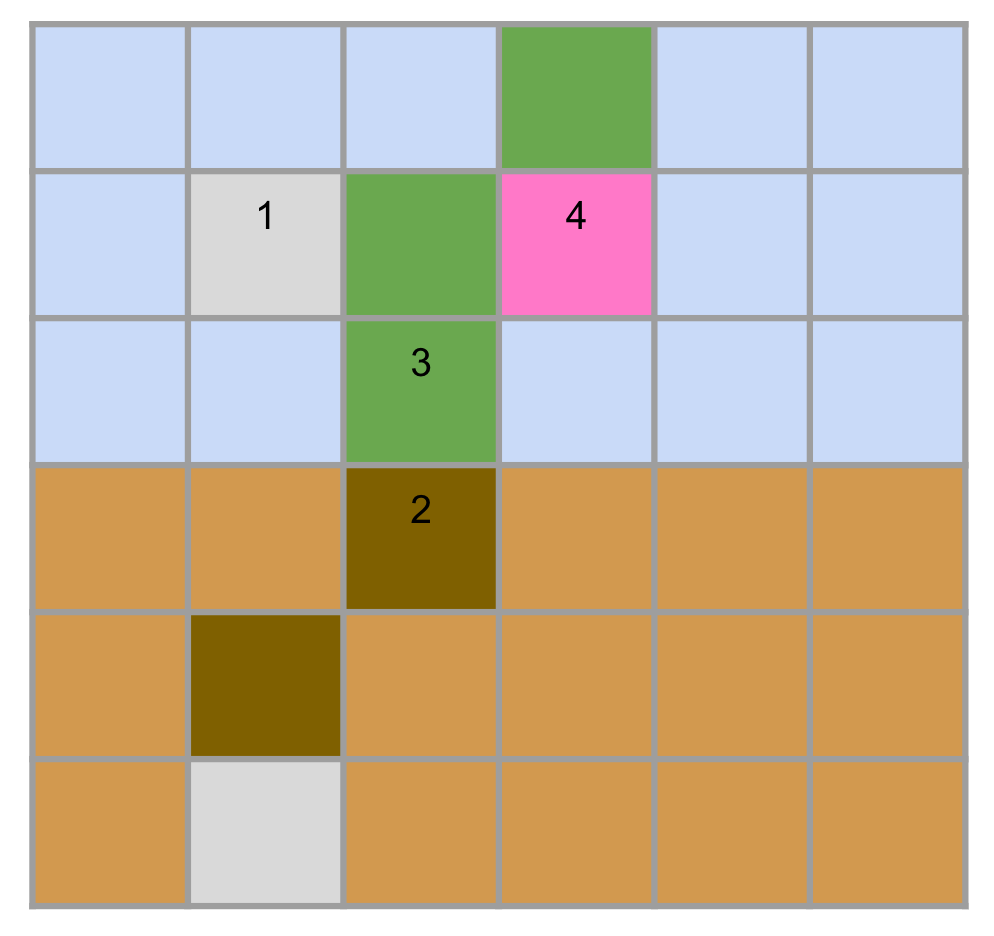
To be fertile, an environment requires at least 5 of these materials:

• Earth, where earth nutrients can be harvested by agent roots.
• Air, where air nutrients can be harvested by agent leaves.
• An Agent type, the materials identifying living cells, each with its own logic and internal states.
• Immovable, the source of earth nutrients and structural integrity.
• Sun, the source of air nutrients.

Also note that the agent cells in the figure above form a "seed". A seed is the initial configuration of an agent organism. An environment starts with a seed, and reproduce operations generate a seed.

Here instead we show a figure with all agent types:

We will explain how the characteristics of all materials are implemented in the system whenever talking about a specific kind of logic.

Every Environment has to be paired with an EnvConfig. This represents the laws of physics of the given environment. The list of parameters is vast and we refer to the code base for an extensive list. But, to get an understanding of the features handled by EnvConfig, here are some: state size, absorption amounts of nutrients, maximum amounts of nutrients, costs of performing any kind of operations for agents and its details, dissipation amounts for agents (how many nutrients agents passively require for maintenance), maximum lifetime of agents.

In this article, we showed four different pairs of Environment and EnvConfig. We called them "configurations", and gave them names (persistence, collaboration, sideways, pestilence). The size of the environment also matters, and in theory we should distinguish between configurations with different sizes, but we chose to simplify the nomenclature and call them all in the same way. However, we will specify their sizes when appropriate. In this article, you will see three different sizes:

• Wide: a very long configuration, generally too large to perform meta-evolution on it.
• Landscape: a 16:9 ratio of a configuration. We mostly use this configuration for evaluations.
• Petri: a smaller version where we slice vertically an environment. This will be paired with a subtle difference in the rules of the environment that we will discuss later on.

Environment logic

Now let's see what operations the environment performs at each step.

Gravity

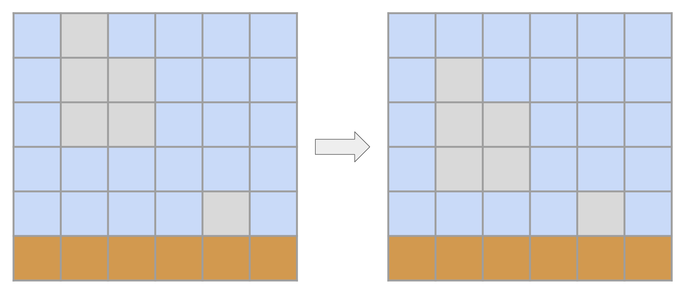
Some materials are subject to gravity and tend to fall down whenever there is an intangible cell below them (with some caveats, as Structural integrity will describe). These materials are Earth and all Agent types. Gravity is implemented sequentially line-by-line, from bottom to up. This means that a block of detached agents/earth will fall simultaneously:

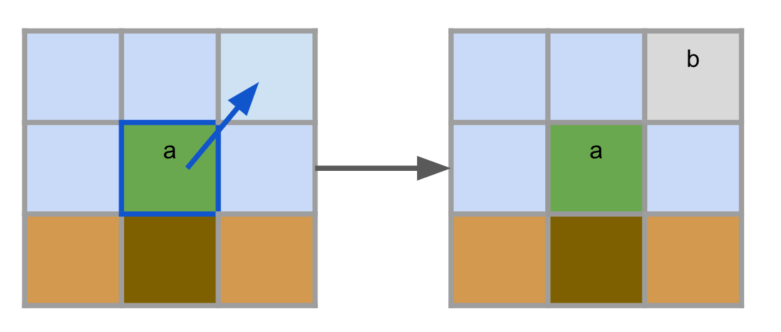
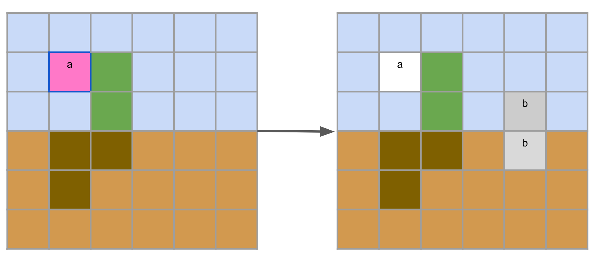
Structural integrity

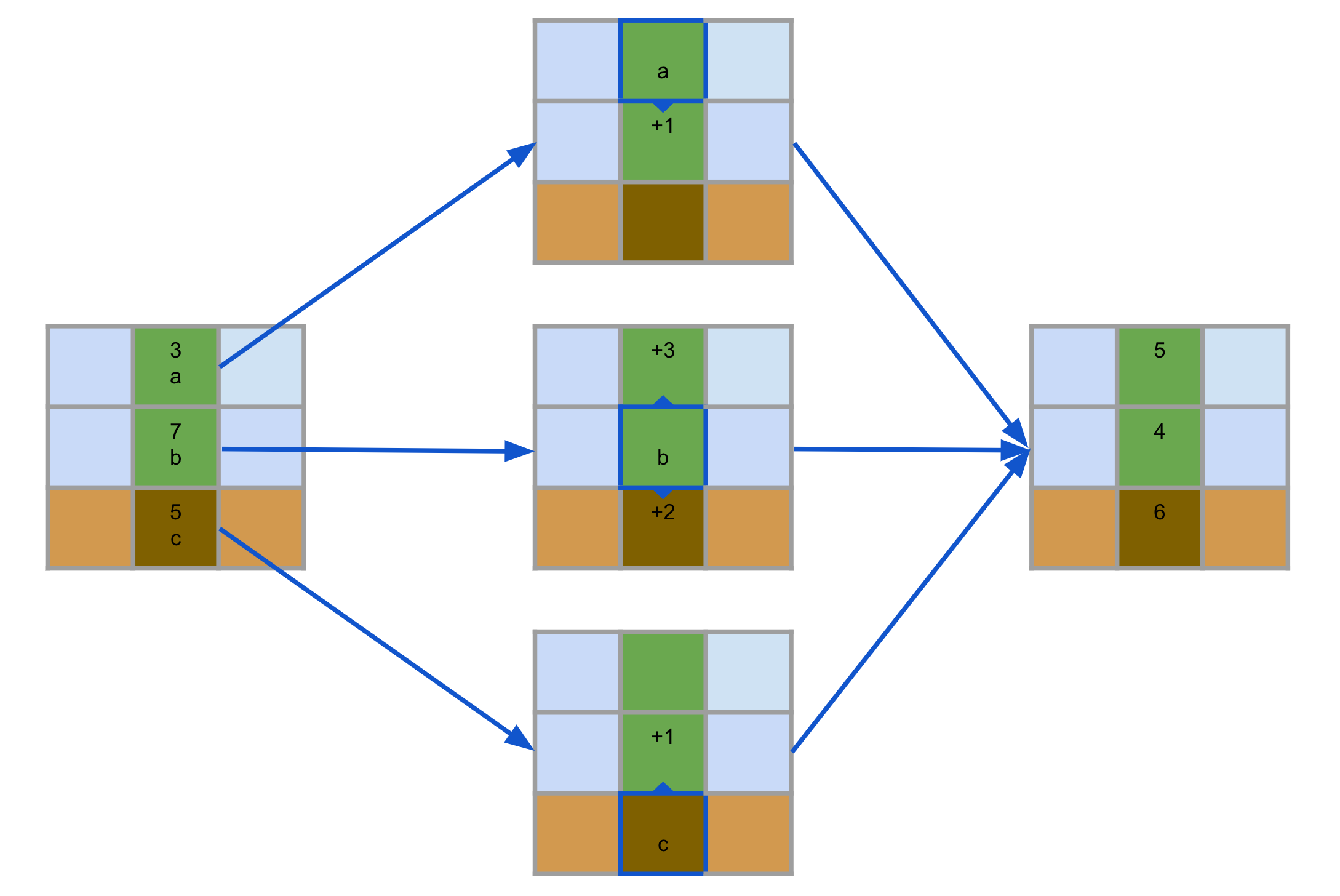
The problem with a simple handling of gravity is that plants couldn't branch out, since they would then fall to gravity. To avoid that, we devised the concept of structural integrity. In its simplest terms, this means that if an agent cell has a nonzero value of structural integrity, it will not be subject to gravity. The way we accomplish this is as follows: Immovable materials constantly generate a very high amount of structural integrity. At every step, each material cell (earth and agents) inherits the highest structural integrity in its neighborhood, decayed by a material-specific amount. For instance, earth may have a decay of 1 and agents of 5, so if the highest value of structural integrity in the neighborhood were 100, an agent would inherit a value of 95. This percolates across all earth and agents and makes it so most tree branches have a positive structural integrity and don't fall.

The figure above shows an example of how structural integrity propagates. Note that earth only propagates structural integrity but is still always subject to gravity, and that if a plant were to be severed during its lifetime, it would take some time for structural integrity to set the cut value's structural integrity to zero. Therefore, we generally perform multiple iterations of structural integrity processing per environmental step.

Aging

At every step, all cells age. This increases a counter in their state values. As the next section will discuss, agents that have lived past their half maximum lifetime will start to dissipate linearly increasing extra energy per step. The only way to reset the aging counter is to reproduce: new seeds (with new agent ids) will have their age counter set to zero.

Energy processing

Immutable and Sun materials constantly generate new nutrients that are diffused to nearby earth and air cells respectively. These cells, in turn, diffuse these nutrients among themselves. This creates an issue of percolation: if an earth/air cell is unreachable by other earth/air cells with nutrients, they will not receive any nutrients. At the same time that nutrients are diffused, roots and leaves neighboring with earth/air cells will harvest a fixed amount of nutrients (if available) from them. Afterwards, all agents dissipate a fixed amount of nutrients. Moreover, if they have reached past their half lifetime, they lose extra nutrients with an ever increasing pace over time. If they don't have enough nutrients, they die. In case of death, if earth nutrients are left, the agent turns into earth. If air nutrients are left, the agent turns into air. Otherwise, the agent becomes void.

Cell operations

Now let's take a look at how we implement the operations of all cells: materials and agents. There are three kinds of operations that cells can perform: parallel, exclusive and reproduce operations.

Parallel operations

These are the operations that can be performed without being concerned with having conflicts with other cells. This includes operations that act on oneself and not on others, or, if they act on others, in a very limited way.

Currently, only agents implement parallel operations, but the energy diffusion operations of materials could be implemented with them as well.

Agents can, at every step:

• Change their own internal states.
• Change their specialization.
• Give nutrients to neighboring agent cells.

There is no restriction on modifying a cell's internal state. However, to change a cell's specialization, the agent needs to have a sufficient amount of nutrients or the operation fails. Finally, giving nutrients to nearby agents naturally cannot generate energy out of thin air, so you cannot give more nutrients than you have.

Exclusive operations

These are the kinds of operations that may conflict with operations performed by other cells at the same time. Generally, these are identified by the fact that they modify a neighboring cell's type. Every cell can only perform one exclusive operation per step (therefore they can only affect one neighbor per step).

Currently, we have three exclusive operations implemented. Air cells spread through void:

Earth cells perform a exclusive variant of the falling-sand algorithm: if they are stacked, and they could fall to either side, they move to the side. Gravity then takes care of making them fall.

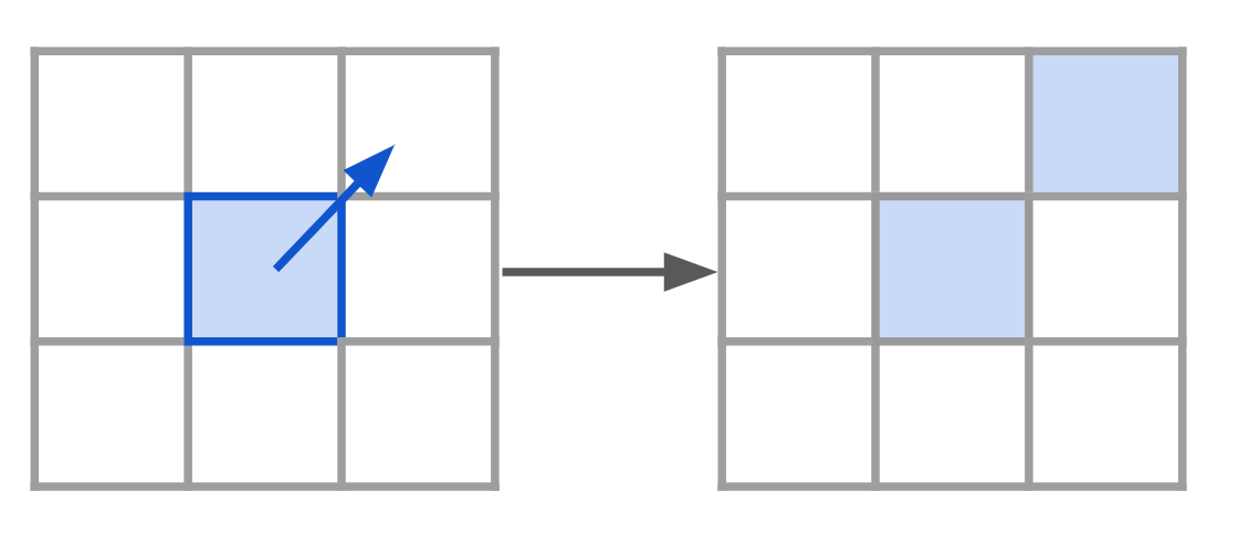
Agents can choose to perform a "Spawn" operation, generating a new unspecialized agent cell in the neighborhood with the same agent's id.

Spawn also has a cost, and it can only be performed on Void, Air and Earth cells. At the moment, this is the only exclusive operation that agents can perform. If we wanted to implement more agent exclusive operations, we would have to make sure that only up to one exclusive operation would be chosen by an agent. In the paper we give more details on how we implement this in the low level, which makes adding new exclusive operations very easy to do.

Reproduce operations

Organisms have to eventually reproduce. They do so by specialising into flowers and trying to perform a reproduce operation. This operation is quite nuanced and there are many details that may cause it to fail, and we refer to the paper for more information. The gist of it, however, is this: if a flower is next to air cells and triggers a reproduce operation, it may succeed. The flower would then be destroyed and a new seed, containing the former nutrients of the flower minus the reproduce cost, may be placed in the neighborhood.

Whenever a new seed is generated, the age of the seed cells is set to zero and a new set of parameters is generated through a mutator (which we will explain later). Therefore, every organism has their unique set of parameters and in-context mutations happen every time a new seed is generated.

Agent logic

Probably the most important design choice that a researcher has to make in Biomaker CA is the choice of the agent logic and its respective mutation strategy (mutator). The agent logic is a set of three different functions and their respective parameters that define the behavior of a given agent with respect to its parallel, exclusive and reproduce operations. All three operations accept the same kinds of inputs: the cell's perception (neighboring types, states and agent ids) and a random number. Their outputs are some interfaces that make sure that no laws of physics can be broken by the agents.

It is very easy to create whatever kind of complex agent logic. Then, we can vectorize it with JAX to run on an entire grid and even multiple environments at a time. However, we want to stress out how hard it is to come up with some agent logic and its respective initialization that would succeed in Biomaker CA. This is because in order to reproduce starting from a seed of two unspecialized cells, the organism needs to at minimum be capable of:

• Specialize accordingly into root and leaf cells.
• Distribute nutrients to neighbors smartly enough to make sure that no cell (or few unimportant ones) dies.
• Perform spawn operations to grow in size and accumulate more nutrients and more importantly create a flower
• Store extra nutrients in the flower and trigger reproduction.

Most initializations and architecture will fail from the start and won't be able to build up anything even through meta-evolution because they would constantly receive zero signals of improvements. We therefore provide two initial agent logics, one with ~300 parameters and one of more than 10000, that are hand-designed to have an initialization that can create fertile plants in most environments.

We chose to hand-write a parameter skeleton to accomplish this goal. This approach is consistent with our perspective that we are more than willing to interact with the environment at specific stages of development if this results in a tremendous speed up in computation or a better resulting complexification. In this article, we will call "minimal" the small architecture and "extended" the larger, since the latter is indeed an extension of the minimal one (it strictly contains more operations and parameters). The minimal architecture does not ever modify an agent's internal states, while the extended architecture can modify them at will and act based on internal states as well.

These architectures are just meant to be crude examples of what is possible and we highly encourage research on what are the best agent logics and their respective mutators.

Mutators

The initial parameters of the agent logic are just the starting point. We can mutate and evolve them in several different ways, but if we want to allow for in-environment mutation through reproduce operations, they must use a mutator. A mutator is a very simple function that takes as input some parameters and a random number, and with that they generate a new set of parameters. This is the function that gets executed whenever a reproduce operation is triggered.

We can roughly distinguish between two kinds of mutators: stateless and stateful. A stateless mutator does not have any parameters by itself. In this article, we refer to "basic" as a stateless mutator that mutates parameters by sampling the new ones from a gaussian with a fixed standard deviation, and has a 20% chance of updating each parameter. A stateful mutator adds parameter to the agent logic. We will instead refer to "adaptive" when using a stateful mutator that doubles the amounts of parameters of the agent logic so that each and every parameter has its own standard deviation for mutation. Each parameter also has a 20% chance of update but crucially also their standard deviation gets in turn randomly updated with a certain chance and standard deviation.

When a mutator generates new parameters, it generates new parameters both for the agent logic and the mutator's. This shows how closely related mutators are to the agent logic. Ultimately, the quest for open endedness and complexification requires to figure out the interplay between modifying a genotype through mutation strategies to result in new genotypes that express interesting new phenotypes.

Note that mutators don't receive extra information such as ranking of a population or fitness values. The only information that they receive is that reproduction was triggered.

Examples and experiments

Reproduce in a Colab

Now that we know how Biomaker CA works, we can start by inspecting some configurations to see how some settings change the behaviour of the environment.

Let's start with "persistence". This environment can have very old agents: the agents' max age is 10000 steps. This means that the agents will always eventually die. Below, we show two runs of persistence. The top row is with the "minimal" setting of agent logic, the bottom row is with the "extended" setting. Both simulations have the same basic mutator (the sd is set to 0.01 and 0.001 for minimal and extended, respectively, since extended has way more parameters).

As you can see, mutations accumulate in wildly different ways. The minimal logic seems very stable even if we are using a higher mutation rate than the extended one. Meanwhile, the extended logic explores a vast array of possible organisms. Disappointingly, these organisms live much shorter lifespans than what is theoretically allowed in this environment. Moreover, we can observe two different evolutionary problems from the two simulations. The minimal configuration doesn't seem to explore nearly enough: the conjunction of genotype and mutation strategy seems to be too conservative. Meanwhile, the extended configuration has the opposite problem: the descendants of the original plant immediately forget how to grow a plant like their ancestor - that is, these mutations seem to forget seemingly good traits over generations.

Regardless of these problems, these configurations work: agents never die out completely. They may not be as pretty as we would want them to, or diverse enough, but they survive, which is a start.

"sideways" has the same EnvConfig of persistence, but the distribution of nutrients is very tricky. This environment may see stable at first, but look at what happens when we let it run for very long:

The environment changes drastically and the biome dies. This shows how the complexity of a configuration can really depend on the environment design as well.

If we wanted to investigate organisms that are potentially immortal, "collaboration" is a good starting point. This configuration has a maximum lifetime of 100 million steps. In practice, agents don't age. However, this is a very costly configuration. Everything is costly: spawn, reproduction, specialization and even dissipation. Therefore, even if you would think that we'd immediately see gigantic plants, that is not the case.

Above we tried 4 different combinations of agent logic and mutators. Cells seem to grow and die out constantly, as they can't figure out how to stabilize and grow slowly. Even if agents are not becoming extinct, the current models are disappointing.

Finally, let's go back to "pestilence". This environment has very low dissipation costs, but the rest is quite costly (spawn, reproduce and specialize). The real issue, though, is its max lifetime of 300. This makes it so that plants die out all the time. As we have seen before, our previous biome on pestilence got extinct. Could different initial configurations fare better?

The extended model with a basic mutator seems to survive. But is this statistically significant? Let us run this configuration a few more times.

Alas, survival of the species seems to be random. It would be nice to have some more control over it. The rest of this article will show methods to accomplish just that.

How to evaluate a configuration

Before we try to improve our models, it would be beneficial to figure out a way to systematically evaluate a configuration. This way, we could compare configurations with ease and perhaps train them through such evaluations. After all, we have just observed how a single run on an environment may give incomplete information, or even be misleading. For instance, is it really true that the extended logic with basic mutators works best on pestilence, or was it just chance?

Well, JAX is fantastic for this. All we need to do is to define an evaluation function and run a configuration to see how it performs. Moreover, we can parallelize this evaluation as many times as we want to have a more statistically significant understanding of how it performs.

What metrics should we care about? For starters, let's say we care about two things: counting the total number of agent cells that are occupied throughout the run; and whether agents go extinct. So, let's do just that for landscape environments for 1000 steps (wide environments are generally too costly to analyse), and let's do 16 runs for each experiment.

The table above shows a wide variety of configurations and their average number of agents present in the environment and their chance of going extinct. As expected, persistence is an easy environment and agents don't seem to ever go extinct. There seem to be the highest number of agents being alive at any time in such configurations. Surprisingly, sideways comes second. This evaluation seems to hint that in 1000 steps there was never an extinction event, however we know that sideways can go extinct, but apparently it only happens on longer time frames. We will investigate this further. Collaboration also seems stable, and we observe extinction only rarely and only with extended models. In these three environments, extended models seem to underperform minimal models. This is undesirable since extended models have a superset of the operations of minimal models, suggesting that our initial configurations are not particularly prone to evolvability.

In pestilence, we clearly see a high extinction rate for all logic and mutator pairs, but all pairs are still able to survive every now and then. It turns out that the extended model with basic mutation was indeed the best setup for this configuration, but it is still clearly not optimal.

The example of sideways clearly shows that this evaluation method may be suboptimal for some configurations. Let's look at an evaluation for sideways only, where we perform 10000 steps.

This evaluation was very costly, but it finally shows that sideways is deceptively hard to solve. Also, it turns out that we chose a very bad agent logic (the extended one) when generating the previous video. The extended logic seems to have a >80% extinction rate in the first 10000 steps. Meanwhile, the minimal adaptive configuration seems to have a low extinction rate. So, let's look at a run that doesn't die out early with this setup:

The results are much better. Alas, even this run eventually dies. But this doesn't seem hopeless. Certainly something can be done there as well.

What to focus on in this article

We have observed several problems in the examples above:

• sideways seems to get extinct after a very long time.
• collaboration is incapable of generating stable lifeforms.
• pestilence gets extinct very often and very quickly.

In this article, we will focus on stopping extinction events on pestilence. This is because we can perform faster evaluations than what would be required for sideways, and because the metric of extinction is much more well defined than the issue observed with collaboration.

From now on, whenever we evaluate some parameters on pestilence, we will evaluate them by running the environments for 1000 steps, since we know that this is good enough for this configuration.

Improving on survivability by extracting successful agents

Reproduce in a Colab

If we want to come up with 'better' initial configurations, how about starting with agents that evolved naturally from the environment? In pestilence, we know that sometimes agents survive. What would happen if we just extracted some of the agents from a developed environment and ran our evaluations against them? This is equivalent to asking: how much are agents becoming more fit, if any, through their in-environment mutations?

So we took a random run that didn't die out of pestilence, with our favourite configuration (extended model with basic mutator), let it run for 6200 steps, and then extracted 16 different programs from agents alive at the end. Below you can see what would happen if we took one of these agents and placed them in a new environment.

Its behaviour is markedly different from our original models. The organisms are much smaller and spawn way more flowers. The biome doesn't die out… but is that just a random chance? What about the other 15? And how do they compare overall with the initial configuration?

In the table above, "default" is the initial configuration that we have already explored in the past, while "extracted" is averaging the results of these 16 different agents extracted after 6200 steps. The evolved agents seem to be consistently better than their random initialization counterparts. They have both evolved to spawn more agents in the long term, and they get extinct much more rarely. In other words, they evolved and became more adapted to the configuration.

End-to-end meta-evolution

Reproduce in a Colab

Since we are using JAX and we have the power of parallelization, it seems natural to ask whether we can "evolve" our initial configurations by explicitly setting a fitness function and evolving through that. In this article we will show two examples of what can be done along these lines.

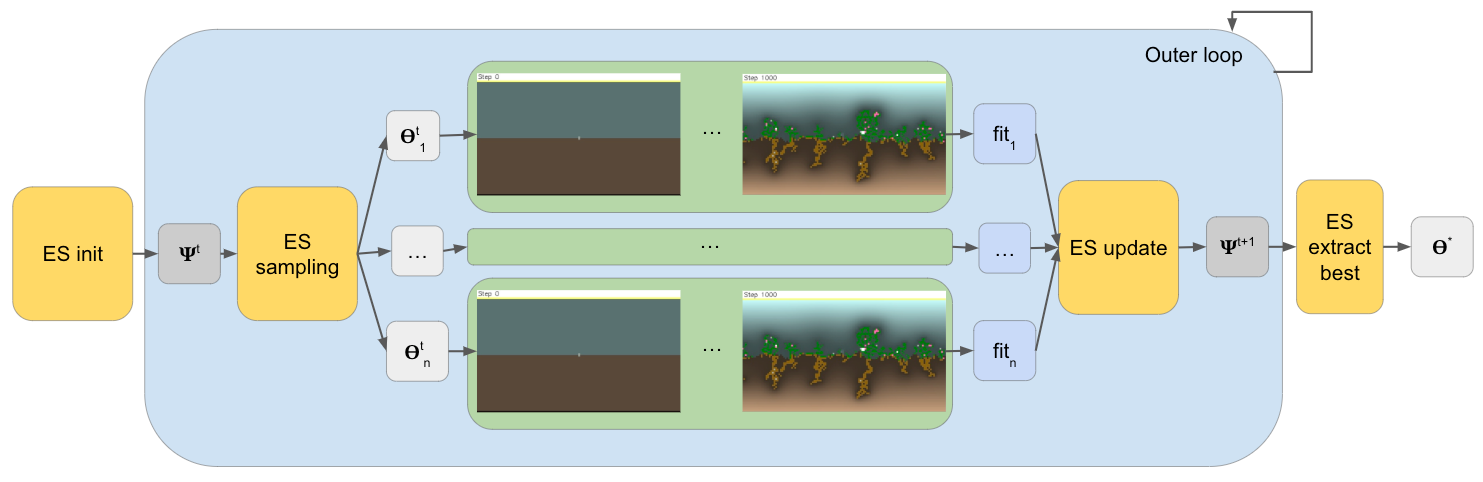
The diagram above summarises meta-evolution. First, we initialize some parameters $\Psi^0$ containing agents initialized parameters and some ES-specific parameters. For each outer step t+1, we sample a population of agent parameters $\Theta^t_i$ using $\Psi^t$. These parameters are each used to simulate a run for several inner steps (1000 in the example). A fitness is extracted by each of these runs and the meta-evolutionary strategy aggregates this information to generate the new parameters $\Psi^{t+1}$. When the outer loop finishes, we extract the best agent parameters $\Theta^*$.

Let's start with end-to-end meta-evolution. Since we are interested in our agents performing well on a landscape width for 1000 steps, and we already have two metrics that we are tracking, we can put these metrics together and run an outer evolutionary strategy where for each example we run a candidate agent for 1000 steps in that environment. Thanks to the system being implemented in JAX, we can use whatever strategy we want to meta-evolve. In this article, we chose to use EvoJAX as a framework, and PGPE as the evolutionary strategy.

Below we show the result of training our extended model with a basic mutator on pestilence for 30 steps with a population size of 32.

And here is how it behaves compared to our previous methods.

Perhaps not surprisingly, training end-to-end gives much better results for the goal that we set it out to optimize. But also for long, out-of-training timelines this model looks very good.

Unfortunately, training this way is quite costly. For instance, using a single GPU, we couldn't have a larger population size, or use adaptive mutation (since it would double the number of parameters stored in memory). Of course, we can always parallelize on multiple GPUs, but let's keep things simple for this article and let's explore what else we can do that is less costly.

Petri dish meta-evolution

Reproduce in a Colab

Instead of performing an environment-wide meta-evolution, we could just focus on a single seed and what it does in its shorter lifetime. We could then evolve a single organism to do what we want it to do, assuming that it would remain isolated in a much smaller environment. For instance, we could want the organism to grow to a certain size and stop growing, and to generate offspring so that it can then be deployed in a real environment.

But how would it "generate offspring" and still remain alone in its environment? That would be breaking the laws of the environment! Well, we can do what we call intercepted reproduction. We create a much smaller environment where the laws of physics are a bit different: when a flower triggers a ReproduceOp, instead of generating a new seed, we destroy the flower and keep track of how much energy the hypothetical seed would have had. If it appears to be "healthy" (it has an amount of nutrients deemed sufficient), we record that a successful reproduction has happened and move on. So, flowers would still die, energy would still be depleted, but no new seeds would appear.

This is what we call Petri dish meta-evolution: separate an agent, place it in a smaller fake environment, evolve it somehow, and then put it back into a bigger, real environment to see how it behaves.

Let's try this approach on pestilence. We can again use EvoJAX and PGPE (this time with a population size of 64) and train a population for 50 outer (meta) steps, where a much smaller environment is executed for 200 steps (agents die after 300 steps at most, but usually they are dead soon before then). The fitness will be determined by trying to maximize the number of successful reproductions while maintaining an agent count of 50 for each inner step. As you can guess, training this is much faster than the previous end-to-end meta-evolution.

Above, to the left is the default configuration in the "petri" world, and to the right is the trained result. You can see how flowers still grow and die, but no new seeds are ever created. Let's see how it performs in the proper "landscape" environment, when reproduction is not intercepted anymore.

This seems to work very well. But what mutator did we even use there? After all, in the "petri" environment, we didn't use any. The video above is with a basic mutator, but adaptive mutators (with reasonable initializations) work just as well:

This training seems to work extremely well, so much so that agents never go extinct. This result may be surprising to some readers: we chose a seemingly arbitrary optimization goal and it transferred well to a different environment with both kinds of mutators (none of which was used during the optimization process). In this case, the reason why this works is likely because our choice of mutators was very conservative to begin with (they don't mutate parameters too much) and because we chose the target of 50 agents in an organism expecting that this would have helped with creating a self-sustaining biome. Essentially, we used our expert knowledge to speed up our research.

This is perfectly fine for our use-cases, but other researchers may disagree and look for more general, expert-agnostic solutions where the agent logic and the mutator are coevolved, while still being in a Petri environment. In the paper version of this article, we discuss why this is harder than one might think, but that it still seems feasible for future work.

Interactive evolution

Reproduce in a Colab

There is one last thing that we want to show which motivated this project in no small amount: interactive evolution. Let's say that you have a model that you think may be very promising for open ended evolution. To not confuse ourselves with nomenclature, a 'model' that can evolve would have to be equivalent to talking about a pair of agent logic and mutator, in this project. So you have a good candidate model (agent logic and mutator). How could you explore its capacity in exploring the phenotypic landscape? How could you tell if this model is too conservative (and nothing really changes) or too extreme (and progress is quickly lost and we can't accumulate complexity)? Besides performing extremely costly and hard-to-inspect experiments, it would be desirable to have a visual understanding of how this model behaves.

There is a famous project called Picbreeder which seems to be perfectly aligned with what we described. In Picbreeder, a user starts from a random initial image or an image of a previous user. The image is iteratively randomly mutated many times and the user selects a new picture to continue the process. That project is about open ended evolution and there is no intrinsic goal that a generic user is expected to have. The user chooses what they please.

We wanted to do the same with Biomaker CA. But also, we can still strive for something while creating our favourite plants. We can try to create organisms that we believe can survive, for instance, or we can study the model to understand its limitations and strengths.

We call our version of Picbreeder "interactive evolution", since what we will look at are not pictures but videos of organisms, and we will still actually aim at creating an organism that can survive. For that, we will again use our "petri" environments with intercepted reproductions and we will randomly mutate agents with a mutator strategy of choice. To be consistent with previous experiments, we will use the extended agent logic with a basic mutator on pestilence. On top of each video there will be written how many successful reproductions they accomplished. The selected offspring will be highlighted in green.

Our thought process with the choice was at first at random, but then our interest was piqued by this organism that in the later stages seemed to explode into many different flowers and then die. We wanted to chase that and this is what happened. Let's see how this agent performs on the real "landscape" environment:

And how does it compare to our other approaches?

The agents never die out and generate a comparable amount of cells with the other approaches. But alas, the explosive property seemed to disappear after a few generations. This shows how we still don't have full control for generating properties that get propagated to all (or most) descendants of a species we engineer. Clearly, there is much more to learn about how to design complex life.

Discussion

Biomaker CA is all about trying out whatever interests you. It is complex enough to allow nontrivial interactions and lifeforms, but simple enough so that progress can be steadily made. Even though we are sure that every person will find something different to try out and explore, let us list some of the things that we see that are possible to explore with Biomaker CA.

First off, what are the laws of physics that stand at the edge of chaos? What universes allow for interesting interactions to occur, and which ones are boring? Would adding new materials and agent operations change that?

What are the best architectures/basic building blocks for creating complex morphogenetic organisms? What mutators work best for evolving quickly into something interesting and potentially arbitrarily complex? Is asexual reproduction enough for it, or should we create a ReproduceOp that is sexual?

How can we design organisms that have key properties that, while they will still evolve in wild ways, won't ever lose these properties?

How can the human be in the loop as much as possible, or as little as possible?

How can we design complex biomes that don't have abrupt extinction events? Can we understand ecology in the real world by simulating biomes in Biomaker CA, or variants of it?

Obviously, there are several limitations that would impede Biomaker CA to generate arbitrarily complex life. One of them is the incapacity of agents to move. Now, we could add a move operation, but the problem is that CA are really not convenient for such a thing: if a cell moves, the rest of the organism doesn't. This may easily break the organisms and we should probably look for different ways to explore moving organisms. Moreover, time is discrete and not continuous, space is likewise. Compositionality of organoids is quite hard in a 2D space, and who knows how many other problems we will discover by exploring its capabilities. Still, we believe that focusing on all the problems that are approachable in Biomaker CA may be the best way to move forward, before we will have the need to create even more complex frameworks.

We hope that this research project may be inspiring to as many people as possible, researchers and observers alike. This is an open project and we warmly welcome contributions or spin-offs of it. There is so much that can be done with Biomaker CA, so much that we don't understand or don't know how to do, that we believe we could all benefit a lot from exploring this framework further.